Learning objectives

• Learn to plot 3D graph to visualize potentials in multidimensional space
• Play around with the generalized force constants of 2D harmonic potential to understand how the diagonal and off-diagonal elements influence the shape of the potential

Background

When we study vibration in polyatomic molecules, we know that we can write down the Taylor expansion of the potential, and if we keep up to the quadratic terms, we can get

\[V= V(0)+ 1/2\sum_{i,j} k_{ij}x_ix_j.\]

Here $k_{ij}$ is the generalized force constant, and $x_i,x_j$ denotes the displacements of the coordinates.

The square terms, $\frac{1}{2}k_{ii}x_i^2$ are fully analogous to the 1D Harmonic potential. The cross terms with $i\neq j$ are more mysterious: what is the physical meaning of the cross terms? How do they influence the shape of the potential?

Find the answer by visualization

One of the most intuitive ways to understand a multi-dimension function is to visualize it. To simplify the discussion, let’s focus on visualizing the 2D harmonic potential.

\[V(x,y)= V(0)+ \frac{1}{2}k_{11}x^2 + \frac{1}{2}k_{22}y^2 + \frac{1}{2}k_{12}xy + \frac{1}{2}k_{21}xy\]

Notice that by definition, $k_{12}=\frac{\partial^2V}{\partial x\partial y}$, $k_{21}=\frac{\partial^2V}{\partial y\partial x}$, we have $k_{12} = k_{21}$. Thus we can further write the 2D harmonic potential as

\[V(x,y)= V(0)+ \frac{1}{2}k_{11}x^2 + \frac{1}{2}k_{22}y^2 + k_{12}xy\]

We can then present the 2D potential in 3D, or 2D contour plot, or 1D plot along direction in the XY plane.

Try and learn

Run the following code blocks to visualize the 2D harmonic potential in different ways and understand how $k_{11}$, $k_{22}$ and $k_{12}$ influence the shape of the potential.

Instructions

• First, click “Activate” to activate the code block.
• Once you see the buttons to “run” at the bottom left corner of the code block, click “run” to run the code.
• Please be patient. Starting the kernel can be slow sometimes.
• You may drag the sliders to change $k_{11}$, $k_{22}$ and $k_{12}$ values.
• To isolate the effects of changing $k_{11}$, $k_{22}$ and $k_{12}$ values, first set $k_{12}=0$, adjust $k_{11}$ or $k_{22}$ and see how the shape of V changes.
• With $k_{11}$ and $k_{22}$ values fixed, adjust $k_{12}$ and see how the shape of V changes.

Activate

1. 3D contour plot

This code block visualizes the 3D contour plot of the harmonic potential. Both the color and the height in Z-direction indicate the potential value. The contour lines represent regions in the (x,y) plane with the same value of V(x,y).

%matplotlib widget
import ipywidgets as widgets
import numpy as np
import matplotlib.pyplot as plt
from mpl_toolkits import mplot3d

def V(x, y, k11, k22, k12):
    return 0.5*k11*x ** 2 + 0.5*k22*y ** 2 + k12*x*y

# Define the interactive widgets

k11_options = widgets.FloatSlider(
    value=1.0,
    min=0.1,
    max=2.0,
    step=0.1,
    description=r'$k_{11}$:',
    disabled=False,
)

k22_options = widgets.FloatSlider(
    value=1.0,
    min=0.1,
    max=2.0,
    step=0.1,
    description=r'$k_{22}$:',
    disabled=False,
)

k12_options = widgets.FloatSlider(
    value=0,
    min=-1.0,
    max=1.0,
    step=0.1,
    description=r'$k_{12}$:',
    disabled=False,
)

y_options = widgets.FloatSlider(
    value=0,
    min=-6,
    max=6,
    step=0.5,
    description=r'$Y$:',
    disabled=False,
)

x_options = widgets.FloatSlider(
    value=0,
    min=-6,
    max=6,
    step=0.5,
    description=r'$X$:',
    disabled=False,
)


theta_options = widgets.FloatSlider(
    value=0,
    min=0,
    max=180,
    step=10,
    description=r'$\theta$:',
    disabled=False,
)

fig = plt.figure()

@widgets.interact(k11=k11_options,k22=k22_options, k12=k12_options)
def update(k11,k22,k12):
    fig.clf()

    x = np.linspace(-6, 6, 30)
    y = np.linspace(-6, 6, 30)

    X, Y = np.meshgrid(x, y)
    Z = V(X, Y, k11, k22, k12)

    ax = plt.axes(projection='3d')
    ax.contour3D(X, Y, Z, 50, cmap='viridis')
    ax.set_xlabel('x')
    ax.set_ylabel('y')
    ax.set_zlabel('V(x,y)');

2. 2D contour plot

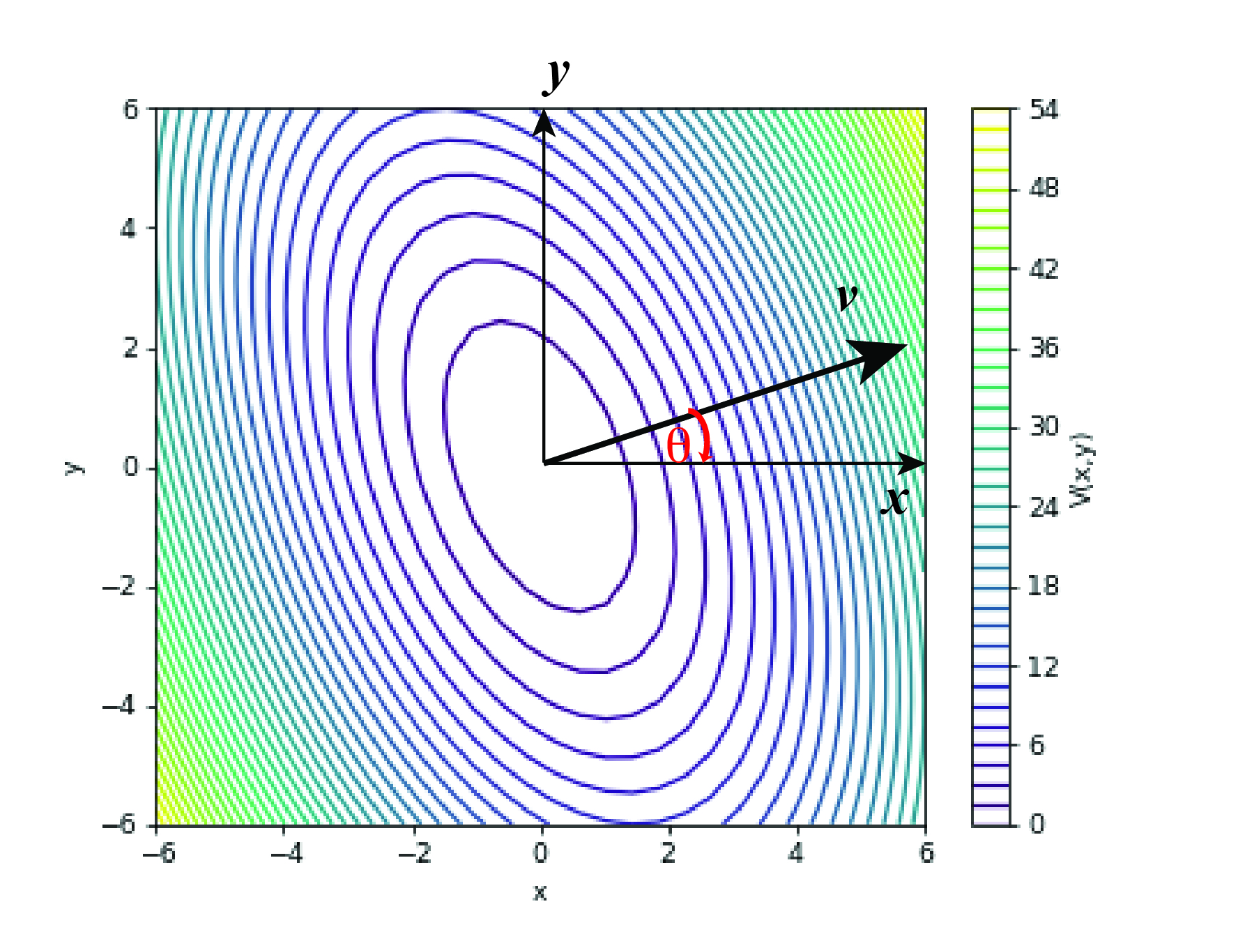
The next code block visualizes the 2D contour plot of the harmonic potential. The color indicates the potential value. The contour lines represent regions in the (x,y) plane with the same value of V(x,y).

fig2=plt.figure()

@widgets.interact(k11=k11_options,k22=k22_options, k12=k12_options)
def update2(k11,k22,k12):
    fig2.clf()

    x = np.linspace(-6, 6, 30)
    y = np.linspace(-6, 6, 30)

    X, Y = np.meshgrid(x, y)
    Z = V(X, Y, k11, k22, k12)

    ax2=plt.axes()

    plt.contour(X, Y, Z, 50, cmap='viridis');
    ax2.set_xlabel('x')
    ax2.set_ylabel('y')
    ax3 = plt.colorbar();
    ax3.set_label('V(x,y)');

3. Value along a line in X-Y plane across the origin.

In the next code block, we want to visualize the V(x,y) value along a line in the X-Y plane across the origin. We can set an angle $\theta$ to denote the direction of the line. Then we plot the V(x,y) value along the line in a 1D plot.

# Then visualize the parabola in the theta=theta_value direction,

fig4=plt.figure()

@widgets.interact(k11=k11_options,k22=k22_options, k12=k12_options, theta=theta_options)
def update3(k11,k22,k12,theta):
    fig4.clf()

    v = np.linspace(-6, 6, 100)
    x = np.cos(theta)*v
    y = np.sin(theta)*v

    z = V(x,y, k11, k22, k12)

    plt.plot(v,z)
    plt.xlabel('v')
    plt.ylabel('V(x,y)')
    plt.ylim(0,50)
    plt.title(r'V(x,y) with $\theta$= {:.1f}'.format(theta))

Questions

1. How does the potential shape change with $k_{11}$?
2. How does the potential shape change with $k_{22}$?
3. How does the potential shape change with $k_{12}$?